Inhaltsverzeichnis
Plot Sheet
Overview
A „Plot Sheet“ component shows diagrams organized in rows and columns of a table, in one or more pages. The count of diagrams, descriptions and the variables to show are configured in a specific xml-file, stored in the „SheetDefs“ subfolder of the project. Very complex definitions are possible e.g. to show different sets of reference data behind the curves, to show markers e.g. an upright line at the position of foot strike in the case of a gait analysis sheet or to compare different groups of patients.
Available features
General
- time-normalized (100%) data, e.g. angels normalized to 100% of a gaitcycle
- xy-plots (e.g. angle-angle diagrams)
- phase-diagrams (normalized angle-velocity over angle)
- diagrams showing continous relative phases (CRM)
- reference data presented as gray bands
- showing events as upright lines
- showing single positions e.g. from static trials as „crosses“
- configurable title of the complete sheet
- configurable titles of each diagram
- showing a legend on the left side of the sheet
- a navigation window to enable/disable or select each phase/cycle
- autoscale or fix scale for each diagram separately configurable
- more than one or two timeseries in each diagram is possible
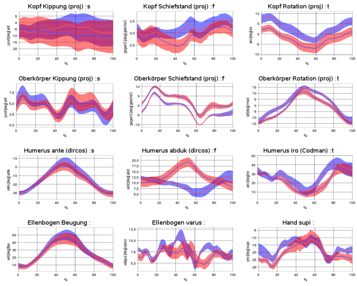
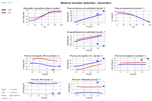 Example sheet with legend on the left side and title on top of the sheet, diagrams show time-normalized and xy-plots and crosses for static measurements. It demonstrates that it is possible not to show at each sheet table position a diagram („holes“ are allowed.).
Open a plot sheet
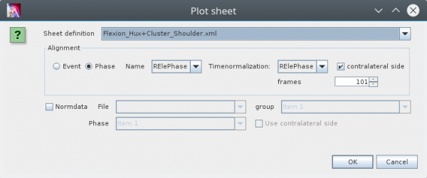
To open a sheet use the the „Plot Sheet“ action in the context menu of single or multiselection of data, e.g. in the tree of an d3d-files. This opens the following dialog:
In the combobox on top you can select the „Sheet definition“. Its the name of an xml file saved in the „SheetDefs“ folder of your project. The following box you can specify how the data should be aligned (splitted into phases and normalized). You can split the data into phases based on events or based on already defined phases in you datasets. In the most of the cases you will split the data phases on predefined phases. Than you can choose this phase in the comobox.
There is an other comobobox to select the phase to use for timenormalization. In the current version you have to set this to the same phase because the functionality of sub-phase-normalization is not yet available.
If your data contains left and right phases you can select the corresponding flag on the right to make the phases of the contralateral side available. This assumes that its phase type names are identical but have a different prefix (R instead of L or L instead of R).
If you want to show reference data as gray band behind your data you can select the corresponding checkbox on the button. In this case you have to specifiy some further infomration about your reference data: First you have to select the file where your reference data is saved. If the combobox does not contain any choice than is no reference data available in the reference data folder of you project. If you have choosed a reference data file you have to define which group and which phase to show. You can show different reference data for left and right sides if you select the corresponding checkbox.
Save Mean+Std-Deviation of selected data
If the sheet shows mean/std-data of selected cycles, e.g. left and right mean stride in the case of a gaitanalysis session, the data can be saved as a .d3d-file into the projects „output“- folder. The saved data file can be used as input for calculation of an inter-subject mean and std data reference, to be shown as gray bars behind the curves.
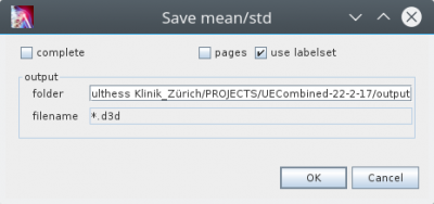
In the Plot Sheets tab context menu, execute “Save Mean/Std” action. This opens the following dialog:
The option „use labelset“ can be used, if you want to export a set of timeseries defined in the project definition, which can be different than the set of timeseries shown in the plot sheet. This is useful, if you have more than one sheetdef to visualize your data but you want to save always the same dataset. To use this feature you have to add a <export>-tag for the calcgroup definition, with an „labelset“-attribute to specify the path to the labelset-file. Have a look at the following example:
<CalcGroup name="ShoulderAnteRetro"
           view="StickFigure.xml">
        <identification>
            <!--entry key="NOTES">ShoulderAbd/Add</entry-->
            <entry key="TYPE">Dynamic</entry>
            <entry key="ACTIVITY">Ante-/Retro</entry>
        </identification>
        <process>
            <entry key="POINTS">true</entry>
            <entry key="EVENTS">true</entry>
        </process>
        <output labelset="Output_reduced_anteretro.xml"
                handlerclass="de.orat.motionDataConverter.MotionDataOutputHandler">
        </output>
        <export labelset="Export_anteretro.xml"/>
</CalcGroup>
If the calcgroup definition is not found, or there is no export definition or the labelset is not found the „use labelSet“ flag is ignoried and the output labelset is defined by the timeseries shown in the labelset.
The idea of the flag „pages“ is to seperate the output into groups defined by the pages of the sheet. For each page a separate mean/std is determined. This is interesting if not for all pages enough phases are available to determine mean/std. The functionality is not yet implemented. The flag is ignored.
If the flag „complete“ is set the flag „use labelset“ and the set defined implicit by the sheet defintion is ignored and all available timeseries are saved.
After pressing the „ok“-button of the dialog a file with the file suffix “.d3d” is saved in the selected folder. Per default its the “output” subfolder of the opened main project. The filename includes the patient id (parent folder name) and delimited with “_” the name of the motion (sub folder name).
The structure of this file is
 <subject>/<session>/<group>/<phase>/<original trial name>_<phase number>
 <subject>/<session>/<group>/<phase>/<original trial name>_<phase number>
 <subject>/<session>/<group>/<phase>/meanStd
 ...
 <group>/meanStd
This means that timeseries of time normalised phases and its mean+std are saved independand from the plot sheets mean or single trials setting. The saved single phases data is indpendand from the phases selection in the sheet. Always all available single phases are saved.
If the shown data does not include enough phases to determine mean/std, than an empty meanstd group is created?
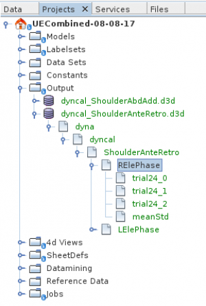
The image above shows the tree-view of such a saved output d3d-file. You can select its „phases“ or groups of phases to plot or to export.
The saved d3d-files can be used to create a reference data set as it is shown as grey bands behind patient data.
Datamining
Extracting of scalar-parameters from the timeseries based on a xml-configuration and saving them into a spreadsheet file e.g. for Microsoft excel or Libre/Open-Office is possible.
In the Plotsheets tab context menu, execute „Datamining“.
Configuration
The main structure of the xml-configuration file looks as follow:
<Sheet name="">
   <Pages>
      <Page rows="" columns="">
          <Diagram name="" .../>
      </Page>
   </Pages>
</Sheet>
Diagram configuration
The table shows the Attributes of the <Diagram> element:
| Attribute name | Default | Description | Required | Comment |
|---|---|---|---|---|
| name | name of the element used to identifiy the element | Yes | ||
| comment | No | |||
| column | Index of the column where the diagram is placed. | Yes | ||
| row | Index of the row where the diagram is placed. | Yes | ||
| xunit | x-axis unit name | No | ||
| yunit | y-axis unit name | No | ||
| diagramDescriptionDown | No | |||
| diagramDescriptionUp | No | |||
| diagramDescriptionLeft | No | |||
| diagramDescriptionRight | No | |||
| plane | s = sagital, f=frontal, t=transversal, typically a shortcut for the plane. | No | The letter is printed in the diagram title after the character „:“. | |
| diagramType | xt | xt, xy, xyz, phase, phaseangle, phaseshift, fft | No | |
| diagramTitle | Text line printed above the diagram followed by „ :“ and the side given with the attribute „plane“. | No | ||
| upperYLimit, upperXLimit | autoadjust | Only if both attributes are set to double values, the upper and lower limit of the diagram is set. | No |
Timeseries Data configuration
Each diagram can plot one or more timeseries. For each diagram a minimum of one <Label>-element is needed, e.g.:
<Label name="RHeadAnteRetroProjAngle"
       component="0"
       side="right"/>
If the timeseries are not of the math type double, the attribute „component“ allows to define, which component should be plotted. The side of the timeserie can be defined by the corresponding attribute.
| Attribute name | Default | Description | Required |
|---|---|---|---|
| name | Name of the timeserie, as used in the data files. | Yes | |
| component | x (==0) | x,y,z if the math type of the timeseries is multidimensional, e.g. 3d vector, 3×3 matrix 3d, quaternion, … an integer number starting with 0 defines, which of the components should be plotted. | No |
| xcomponent | x (==0) | x,y,z component attribute corresponding to the referenced xLabel | No |
| ycomponent | y (==1) | x,y,z component attribute corresponding to the referenced yLabel | No |
| zcomponent | z (==2) | x,y,z component attribute corresponding to the referenced zLabel | No |
| side | not set, which is interpreted most as „both“. | left, right, both | No |
| label | not set | Name of the timeserie as used in data files which includes all the needed dimensions. If not set, the value of the name attribute is used instead. | No |
| xlabel, xlabel, zlabel | not set | For multidimensional plots as alternative to the label or name attribute, if the timeseries are saved as one-dimensional trajectories. | No |
| xmean, ymean | false | Used for xy-plots only: If set to „true“ the corresponding timeserie (defined by xlabel and xcomponent or yLabel and yComponent) is averaged and only the mean (const) value is used. If both attributes are set to „true“ than a point is shown, else a horizontal/vertical line. | No |
| xstartvalue, ystartvalue | false | If set to „true“, than the value of the timeserie at index=0 is subtracted from all frames. This can be used in combination with xoffset. | No |
| xoffset, yoffset | 0 | Name of a variable. Its value is added. If the variable is a timeserie the value at index=0 is used. | No |
| xoffsetcomponent, yoffsetcomponent | 0 | If the variable defined by the attribute offset is multideminsional than this attribute defines the component to use. | No |
| xsign, ysign | false | If set to true, than the sign of the timeserie is reversed. This processing step is done before offset/startvalue processing!!! | No |
If the attributes xLabel, yLabel, zLabel are used, the attribute „component“ is ignored. Instead the attributes xComponent, yComponent and zComponent are used.
The <Label>-element can have <Filter>-children to show filted data as described here.
Data groups configuration
<Sheet>
   <Groups>
       <DefaultGroup name="" leftColor="" rightColor="" normData="">
           ...
       </DefaultGroup>
       <Group name="" leftColor="" rightColor="" normData="">
          <identification>
              <PropertyGroup name="">
                  <Property key="" value=""/>
                  ...
              </PropertyGroup>
          </identification>
        </Group>
   </Groups>
</Sheet>
The following table shows the attributes of of the <Group> and <DefaultGroup> elements:
| name | Description | Required |
|---|---|---|
| name | group name | No |
| leftColor | color name for left side curves | No |
| rightColor | color name for right side curves | No |
| normData | name of the norm data file | No |
Reference Data
Without a specific configuration for each <Label>-element child of a <Diagram>-element in the reference data file is searched for a data set with the name name. E.g. for gait data only one gray band for left and right side should be shown. For this a specific reference data configuration is needed. Have a look at the following example:
<Diagram name="ABC">
 ...
 <Norm name="NORMPelvisAngles"
        component="0"/>
</Diagram>
It is assumed that the normal data file includes a timeserie with the name NORMPelvisAngles with mean and standard deviation. In the unusal cases where mean and standard deviation has different label names the following syntax with additional attributes is possible. But this is not recommended.
<Norm name="NORMPelvisAngles"
       component="0"
       mean="NORMPelvicTilt"
       std="NORMStdPelvicTilt"/>
| Attribute name | Description | Required |
|---|---|---|
| name | Name of the timeserie. If there are no optional attributes „mean“ and „std“ this is also the name of the timeserie searched in the normal data file, including mean and standard deviation. | Yes |
| component | If the math type of the timeseries is multidimensional, e.g. 3d vector, 3xd matrx, quaternion, … an integer number starting with 0 defines which of the components should be plotted. | No |
| mean | For the unusal case that there are saved seperate timeseries for mean and standard deviation. This defines the name of the timeserie for the mean. (not recommended) | No |
| std | For the unusal case that there are saved seperate timeseries for mean and standard deviation. This defines the name of the timeserie for the standard deviation. (not recommended) | No |
Example
<?xml version="1.0" encoding="iso-8859-1" ?>
<?DOCTYPE Sheet PUBLIC "-//Nimue//DTD Sheet Def 1.0//EN" "sheetdef_1.0.dtd"?>

<Sheet name="FullBodyKinamtikPIGCloneAngles">
 <Pages>

    <!-- upper extremity angles -->
    <Page name="upper extremity angles" rows="4" columns="3">

       <!-- Head -->
       <Diagram name="HeadTilt"
                column="0"
                row="0"
                unit="deg"
                diagramDescriptionDown="post"
                diagramDescriptionUp="ant"
                plane="s"
                diagramType="xt"
                diagramTitle="Kopf Kippung (proj)">

                <Label name="RHeadAnteRetroProjAngle"
                       component="0"
                       side="right"/>
                <Label name="LHeadAnteRetroProjAngle"
                       component="0"
                side="left"/>
       </Diagram>
       <Diagram name="HeadObliquity"
                column="1"
                row="0"
                unit="deg"
                diagramDescriptionDown="gegenS"
                diagramDescriptionUp="gleicheS"
                plane="f"
                diagramType="xt"
                diagramTitle="Kopf Schiefstand (proj)">
      ...
    </Page>
  </Pages>
</Sheet>
Options
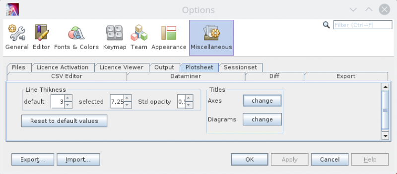
In the Options panel, you can find it in the Tools menu there is a PlotSheet tab to configure the linethikness of the plots and the font used for the diagram title.
Notes
How to plot a parameter as a line
Paramters are saved externally in a non trial-based file. To plot such a parameter as a line, a timerserie is needed in a trial. This can be achived by:
<Real name="ABC"
              calibrateIncludes="static_calibrate"
              includes="dynamic">ABCParameter</Real>
„ABCParameter“ is the name of the parameter saved in the session-wide parameter file, e.g. with suffix „.mp“. „ABC“ is the name of the newly created timeserie.
